1  Introduction

1.1 Acknowledgments

Thanks to Marie Postel and Nicolas Lantos for their careful proofreading of the first version of this manuscript and for many corrections and suggestions. Special thanks to Johann Faouzi and Louis Thiry.

Thanks also to the members of the Sorbonne University pedagogical teams who used these exercises for their feedback and contributions: Mathieu Barré, Constantin Bône, Jules Bonnard, Cédric Boutillier, Thibault Cimic, Jeanne Decayeux, Cécile Della Valle, Guillaume Duboc, Jean-Jil Duchamps, Jean-Merwan Godon, Elise Grosjean, Cindy Guichard, Sidi-Mahmoud Kaber, Nicolas Lantos, Mathieu Mari, David Michel, Leo Miolane, Anouk Nicolopoulos, Arnaud Padrol, Diane Peurichard, Marie Postel, Xavier Poulot-Cazajous, Alexandre Rege, Othmane Safsafi, Emmanuel Schertzer, Agustín Somacal, Didier Smets, Robin Strudel, Gauthier Tallec, Nicolas Thomas, Paul Vernhet, Jules Vidal, and Raphaël Zanella.

Finally, I would like to thank the students who worked on these exercises for their constructive feedback, which contributed to the improvement of this collection.

The attentive reader is thanked in advance for pointing out typos or other errors.

1.2 Why Python?

Python is a general-purpose interpreted programming language that has the particularity of being very readable and pragmatic. It has a very large base of external modules, especially scientific ones, which makes it particularly attractive for programming mathematical problems. The fact that Python is an interpreted language makes it slower than compiled languages, but it ensures a great speed of development which allows humans to work a little less while the computer has to work a little more. This particularity makes Python one of the main programming languages used by scientists.

1.3 Prerequisites

This book does not aim to explain the syntax and principles of the Python language, so the prerequisite is to know the basics. There are many resources to update yourself if needed, for example:

• the online course Python Programming MOOC by the University of Helsinki;
• the book Python for Everybody by Charles R. Severance;
• various online courses, like Crash Course on Python.

Moreover, the realization of the exercises requires access to a computer or an online service with Python 3.6 (or more recent) completed by the following modules: NumPy, SciPy, SymPy, Matplotlib, Numba, NetworkX, and Pandas. The use of a code editor allowing writing in Python is also highly recommended. It is suggested here to use Jupyter Lab, which allows both the writing of interactive notebooks and scripts and also the addition of one’s own solutions below the statements, which is very practical. It is not necessary to use Jupyter Lab, other environments are also suitable, such as Spyder or Jupyter Notebook.

The following sections describe how to install and run the Python environment or use it online without installation.

1.4 Documentation

It is generally not useful (nor desirable) to know all the functions and subtleties of the Python language for occasional use. However, it is essential to know how to use the documentation efficiently. The official documentation is available at https://docs.python.org/. The language and version can be selected in the upper left corner. It is strongly recommended to look at how the documentation is written and to learn how to use it.

1.5 Installation

People who cannot or do not want to install Python can go directly to Section 1.6 for alternatives available online without installation.

There are basically three ways to install Python and the modules required to perform the exercises:

• Miniforge is a Python distribution manager. The modules required for the exercises must be installed manually. This is the preferred method on Windows or MacOS.
• Linux repositories: Most Linux distributions allow you to install Python and the core modules directly from the package repositories that come with them. This is the preferred method under Linux.
• Virtual environment: allows you to manage several versions of Python and its modules. This method provides finer and more advanced control over the installed modules than the previous methods.

1.6 Launch of Jupyter Lab

echo "c.NotebookApp.use_redirect_file = False" >> ~/.jupyter/jupyter_notebook_config.py

1.7 Use of Jupyter Lab

Once Jupyter Lab is launched, the window shown in Figure 1.1 should appear in a browser.

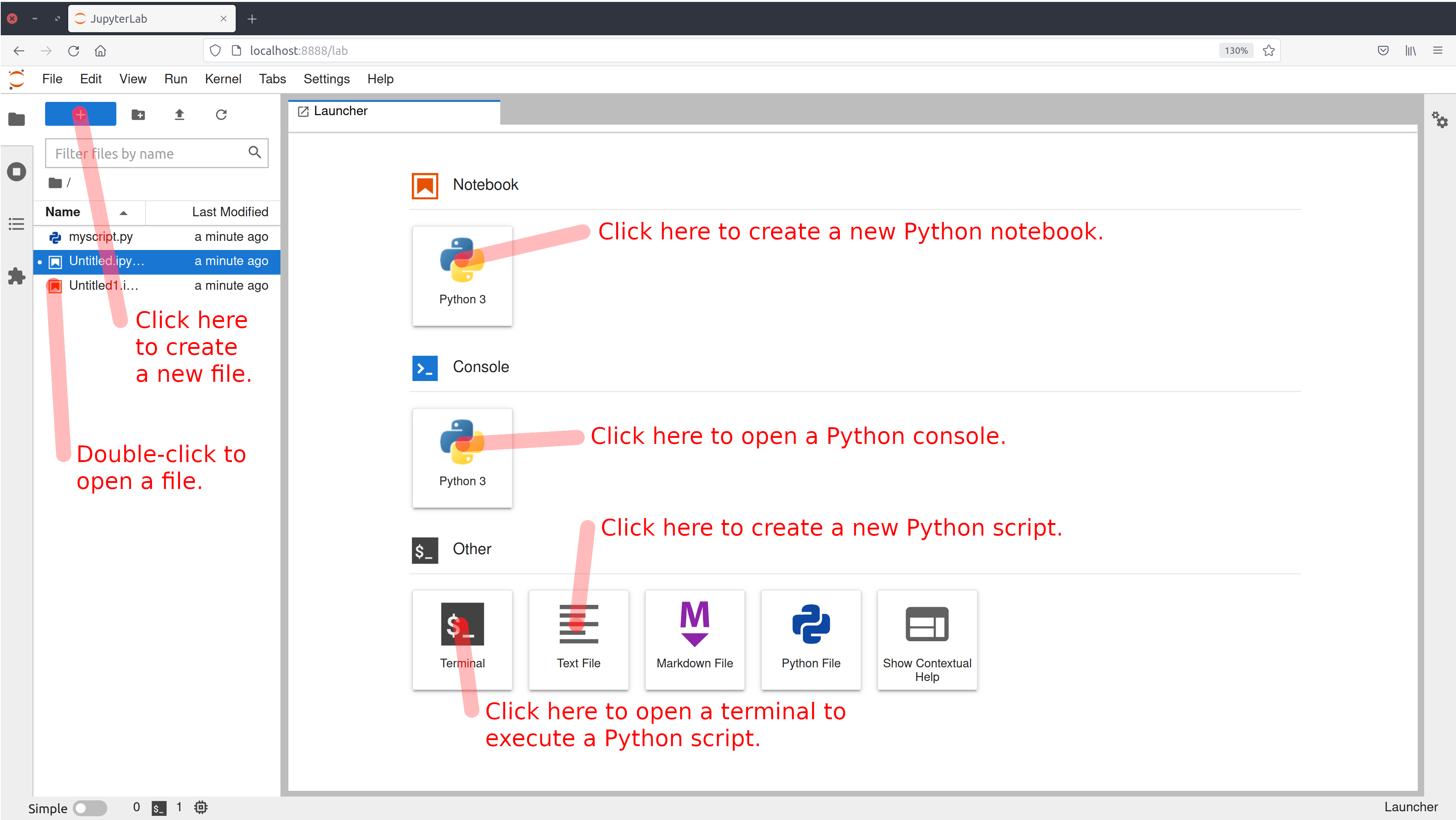
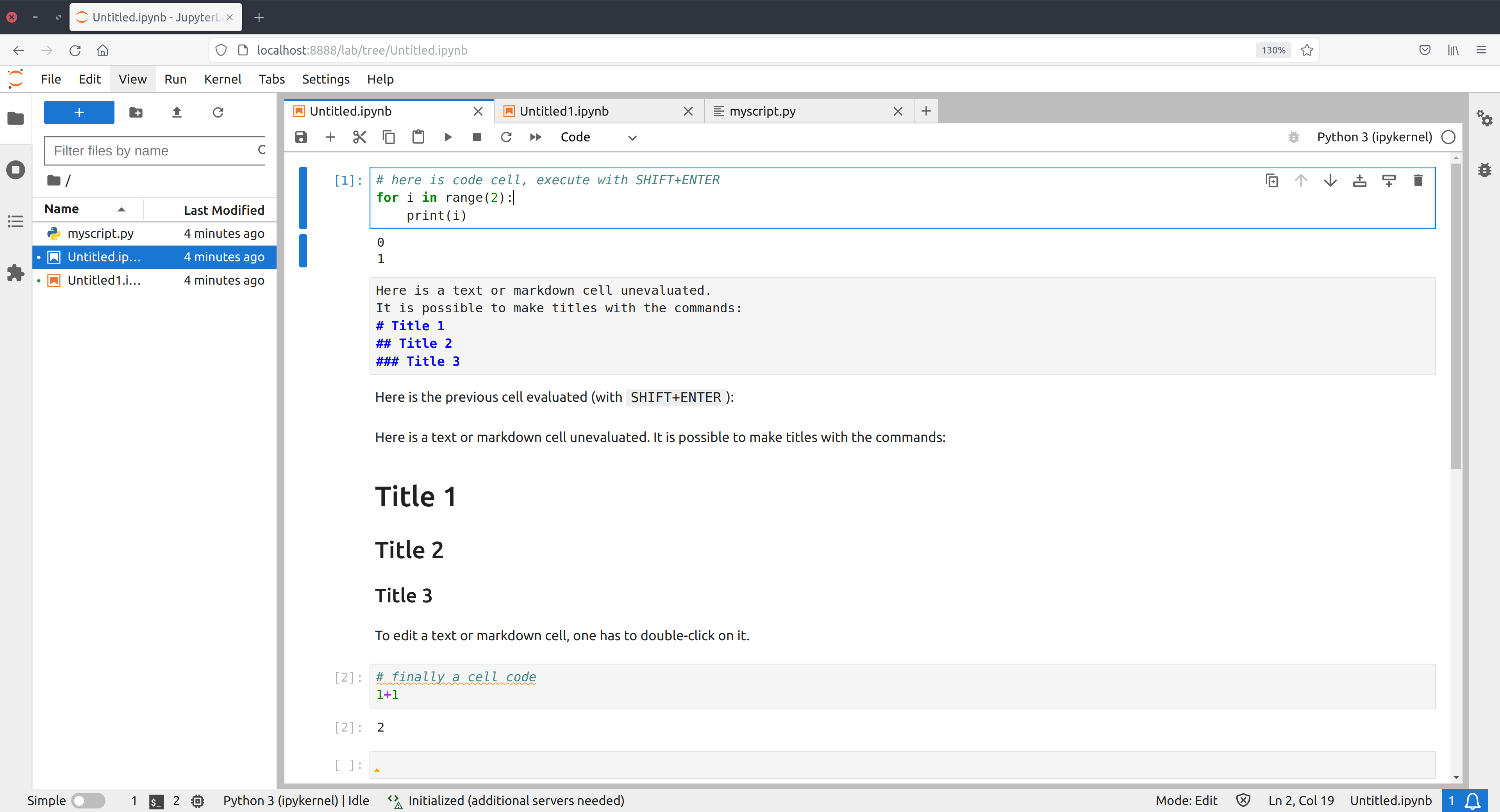
Jupyter Lab essentially allows us to process three types of documents: notebooks, scripts, and terminals. A notebook consists of cells that can contain either code or text in Markdown format. Code cells can be evaluated interactively on demand, which allows great flexibility. Text cells can contain comments, titles, or LaTeX formulas as represented in Figure 1.2.

A Python script is simply a text file containing Python instructions. It is executed in its entirety from A to Z and it is not possible to interact interactively with it during its execution (unless it has been explicitly programmed). To execute a Python script, it is necessary to open a terminal.

Basic commands

• Create a new file: click on the “+” button on the top left, then choose the type of file to create.
• Rename a file: click with the second mouse button on the title of the notebook (either in the tab or in the file list).
• Change cell type: drop-down menu to choose between “Code” and “Markdown”.
• Execute a code cell: combination of keys SHIFT+ENTER.
• Format a text cell: combination of keys SHIFT+ENTER.
• Edit a text cell: double-click on the cell.
• Run a script: type python scriptname.py in a terminal to run the script scriptname.py.
• Rearrange cells: click and drop.
• Juxtaposing tabs: click and drop.

The detailed documentation of Jupyter Lab is available here.

1.8 Advanced use of Jupyter Lab

Recent versions of Jupyter Lab (3 and higher with ipykernel greater than 6) feature a particularly useful debugger and LSP (Language Server Protocol) interface. The debugger allows you to find errors in the code by stopping the program at particular points to understand what’s going on. Documentation and a tutorial on how to use the debugger are available here. The LSP interface provides access to documentation and function signatures, offers code diagnostics and autocompletion. Information on installing and using the LSP interface is available here.

Debugger When writing code, it’s natural to make mistakes, and one important aspect is to locate and identify them efficiently. To do this, it’s possible to put print commands in the right places, but it’s more appropriate to use a debugger for this. To activate Jupyter Lab’s debugger, click on the beetle in the top right-hand corner so that it turns orange. When the debugger is activated, the list of global variables is available in the dedicated bar. The most useful aspect of the debugger is the definition of breakpoints, which allow you to execute the code up to a certain line and inspect the state of the program at that point. To do this, consider the following function, which adds two numbers:

def add(a, b):
    res = a + b
    return res

Clicking to the left of a code line number places a breakpoint indicated by a red dot. Here, we propose to click on the second line performing the addition. By executing the following function call code:

resultat = add(1, 2)
print(resultat)

3

the program will stop at the second line of the add function. You can view the values of variables a and b in the “Variables” tab and the relevant source code in the “Sources” tab. Breakpoints are grouped together in the “Breakpoints” tab. By navigating the “Callstack” tab, you can continue program execution up to the next breakpoint.

Hover When hovering over any part of the code with the mouse, if a part of the code becomes underlined it is then possible to get information about the function with the CTRL key. For example, by hovering the mouse over the following code:

from numpy import linalg

and by pressing the CTRL key with the mouse on numpy or linalg a window with explanations about these modules is displayed. This is also the case for manually defined functions if they contain a docstring:

def square(x):
    """Definition of the function x -> x^2"""
    return x*x

Moving the mouse over the word square:

r = square(4)

underlines it, and with the key CTRL the definition appears.

Diagnostics Critical errors or warnings are indicated by an underline in red or orange, for example, in the case of an undefined variable:

def f(x):
    if x:
        undefined_variable
    return x

Suggestions By typing linalg. in a cell, suggestions of functions available in this module are displayed. In other cases, the suggestions are activated with the TAB key. This is the case, for example, with a manually defined dictionary:

dic = {'key1':3, 'key2':5}

By typing dic[ in a cell followed by the TAB key, the suggestions 'key1' and 'key2' come up.

Signatures By typing linalg.solve( then comes the help and signature of this function, i.e., the way the arguments are to be used in this function. By placing the mouse on the word solve with the CTRL key, there comes also a description of the function.

References By clicking on a symbol, its other uses are highlighted.

Definition By clicking with the right mouse button on a symbol and then on “Jump to definition”, it is possible to go to the definition of the function in question. It is possible to test on the following code for example:

f(None)

Renaming It is possible to rename a variable intelligently (i.e., without renaming local variables, for example) by right-clicking on the variable in question and selecting “Rename symbol”.

Diagnostics panel It is possible to sort and navigate through the diagnostics using the “Diagnostics panel”. To open it, simply select “Show diagnostics panel” from the context menu of a cell (right mouse button).

Personalization The “Settings” menu of Jupyter Lab allows you to customize the working environment, especially to choose the theme, the font size, the default indentation, but also many other more advanced options.