4  Plotting

Exercise 4.1 - Plots

For example, the function plot can be used to represent the function \(x^2\):

x = np.linspace(0,1,50)
y = x**2
plt.plot(x,y)
plt.show()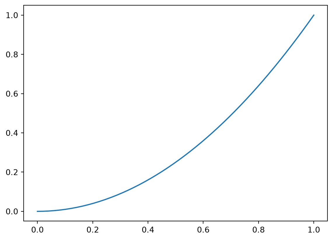

In order to define a nice figure that can be exported as in Figure 4.1, the syntax is as follows:

plt.figure(figsize=(8,5)) # size of the figure (in inches)
plt.title(r'Plot of $x^2$') # title of the figure (LaTeX code can be included)
plt.xlabel(r'$x$') # label of the horizontal axis
plt.ylabel(r'$y$') # label of the vertical axis
plt.plot(x, y, marker='o', label=r"$x^2$") # legend
plt.legend() # display the legend
plt.savefig("test.pdf") # export the figure to PDF
plt.savefig("test.png", dpi=100) # export the figure to PNG
plt.show()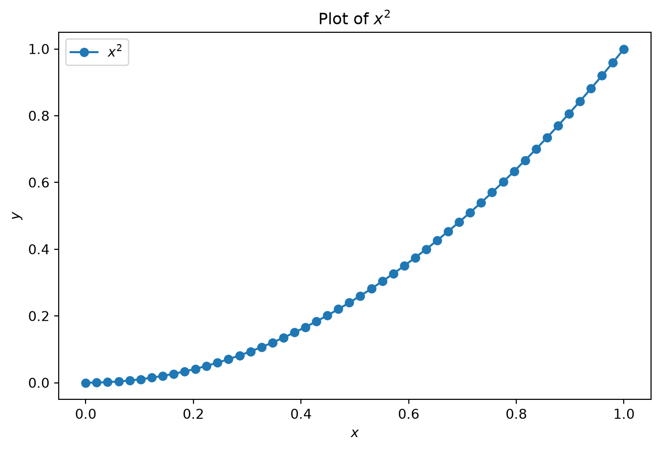

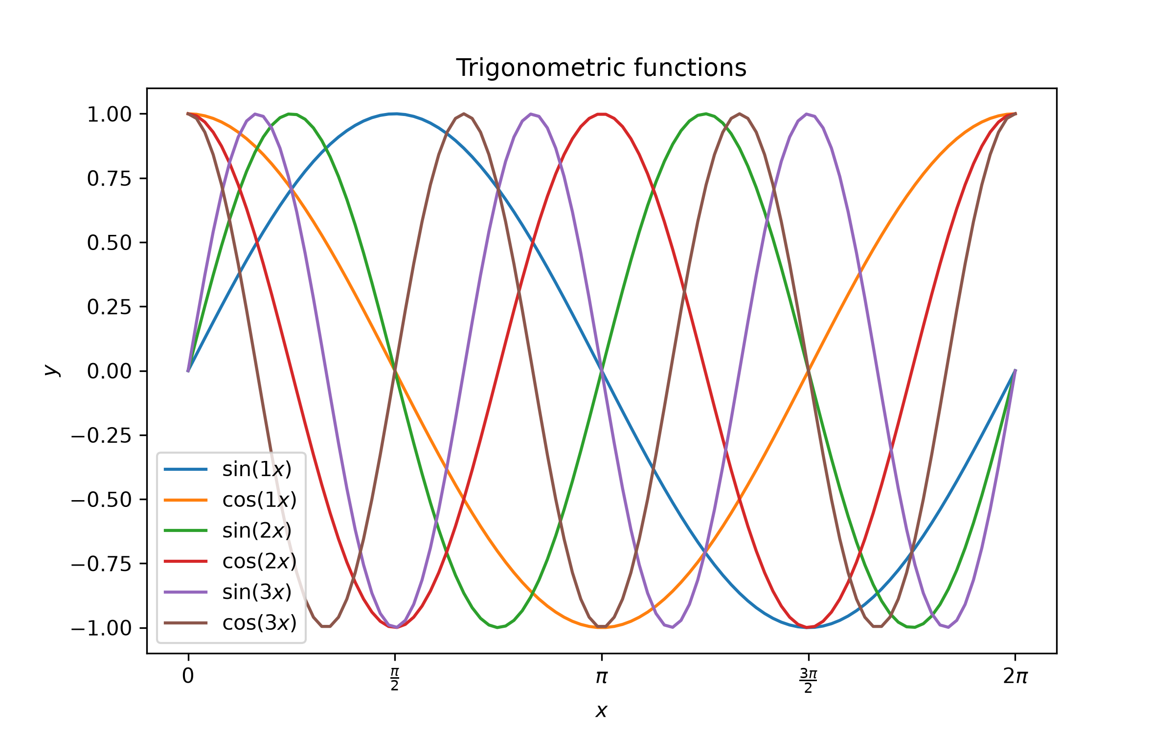
a. Plot the functions \(\sin(kx)\) and \(\cos(kx)\) for \(k=1,2,3\) on \(x\in[0,2\pi]\) in the same figure. Make the graduations on the horizontal axis all \(\frac{\pi}{2}\), as in Figure 4.2.

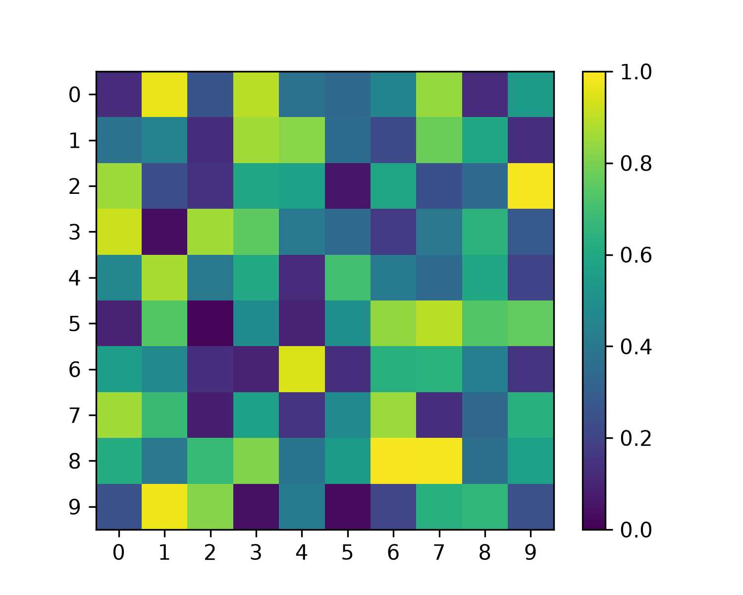
b. Look at the help for the imshow function and use it to plot a matrix of random numbers in \([0,1]\) of size \(10\times10\) as in Figure 4.3.

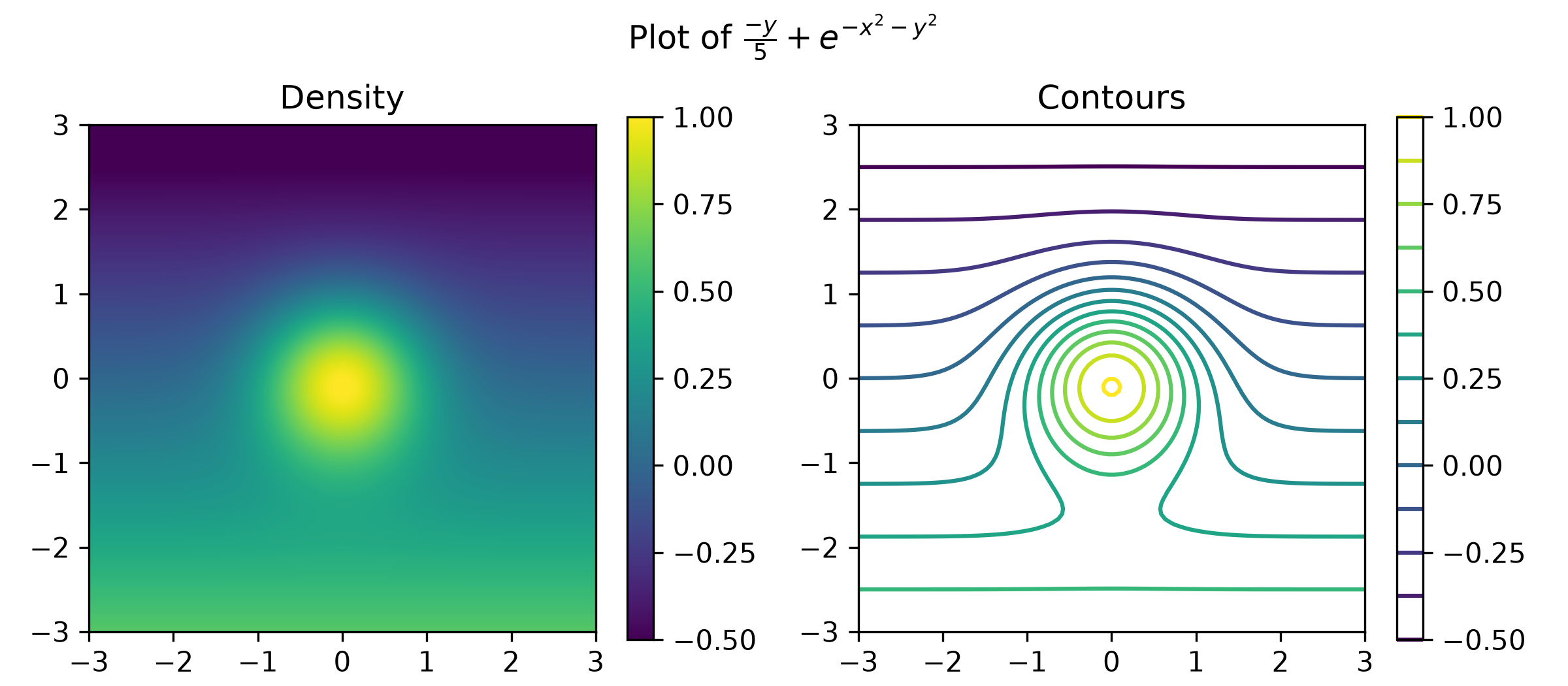
c. Plot the density and the contour lines of the function \(f(x,y) = \frac{-y}{5} + e^{-x^2-y^2}\) for \(x\in[-3,3]\) and \(y\in[-3,3]\) as in Figure 4.4.

Exercise 4.2 - Deterministic chaos

The goal is to study an extremely elementary model of evolution of a population. In spite of its simplistic character, this model presents many very interesting properties, in particular chaotic ones.

The proportion of a population at a discrete time \(i\in\mathbb{N}\) is noted \(x_{i}\in[0,1]\). The evolution of the population is given by \(x_{i+1}=f_{\!\mu}(x_{i})\), where \(f_{\!\mu}:[0,1]\to[0,1]\) is the function defined by:

\[ f_{\!\mu}(x)=\mu x(1-x) \,. \]

The parameter \(\mu\in[0,4]\) describes the population growth. The application \(f_{\!\mu}\) is called the logistic map of parameter \(\mu\).

a. Define the function \(f_{\!\mu}\) in Python as \(\mathtt{f}(\mathtt{x},\mathtt{mu})=f_{\!\mu}(x)\) and plot it for several values of \(\mu\).

b. Why can’t the value of \(\mu\) be greater than 4 in the model?

c. Define a function that takes as argument a value of \(\mu\), an initial data \(x_{0}\in[0,1]\) and a number \(n\in\mathbb{N}\) and returns the list \(S_{\mu}^{n}=(x_{0},x_{1},x_{2},x_{n})\). Modify this function so that it can take an optional parameter \(m\in\mathbb{N}\) and return the list \(S_{\mu}^{m,n}=(x_{m},x_{m+1},\dots,x_{n})\), i.e, remove the first \(m-1\) elements from \(S_{\mu}^{n}\).

d. Test this function by making a graphical representation of the list \(S_{\mu}^{n}\) for different values of the parameters \(x_{0}\) and \(\mu\). Observe the different behaviors of the sequence.

Cobweb diagram. One way to study more specifically what happens when \(\mu\) varies is to make a cobweb diagram that consists in connecting by straight lines the points:

\[ \bigl\{(x_{0},0),(x_{0},x_{1}),(x_{1},x_{1}),(x_{1},x_{2}),(x_{2},x_{2}),\dots,(x_{n},x_{n}),(x_{n},x_{n+1})\bigr\} . \]

e. Define a function that returns the list of points needed to build the cobweb diagram.

f. Define a function that draws the graph of the function \(f_{\!\mu}\), the graph of the identity function, as well as the segments connecting the points of the previous list.

g. By experimenting, study qualitatively the effects of the parameters and \(x_{0}\). Describe the behavior observed when \(\mu\) increases.

Bifurcation diagram. The previous experiments suggest that the behavior of the sequence \(x_{i}\) in large time (i.e., when \(i\) is large) is independent of the choice of the initial condition \(x_{0}\) but depends a lot on the value of the parameter \(\mu\). The aim of this section is to represent graphically for each value of \(\mu\) the set of points \(S_{\mu}^{m,n}=(x_{m},x_{m+1},\dots,x_{n})\), i.e., by putting \(\mu\) on the horizontal axis and all the values of \(S_{\mu}^{m,n}\) on the vertical axis. A good choice of parameters to clean up the diagram and keep only the long-time behavior of the system is \(n=200\) and \(m=100\), for example.

h. Define a function that for a given list \(L\) of values of \(\mu\), an initial data \(x_{0}\in[0,1]\) and integers \(m,n\in\mathbb{N}\) returns the list of points \(\bigl\{(\mu,x):x\in S_{\mu}^{m,n}\;\text{for}\;\mu\in L\bigr\}\).

i. Define a function that plot this list of points. It is suggested to take for \(L\) a list of 1 000 values in the interval \([0,4]\).

j. Interpret the obtained diagram, in particular what it says about the long-time behavior of the system. Determine approximately for which values of \(\mu\) the system :

• has zero as its only fixed point;
• has a unique nonzero fixed point;
• oscillates between two distinct values (cycle of length two);
• oscillates between four distinct values (cycle of length four);
• oscillates between three distinct values (cycle of length three).

Representation of the attractor. For values of \(\mu\) close to 4, the values of the population \(x_{i}\) seem to be more or less random. However, the system is purely deterministic in the sense that for a given initial value \(x_{0}\), the population \(x_{i}\) is defined without randomness. This a priori random behavior is called deterministic chaos. In order to notice that the points \(x_{i}\) are not randomly determined, the goal is to represent graphically the points \((x_{n},x_{n+1})\) to see that \(x_{n+1}\) is not random at all with respect to \(x_{n+1}\).

k. For each given value of \(\mu\), define a function that returns the list of points:

\[ \bigl\{(x_{m},x_{m+1}),(x_{m+1},x_{m+2}),\dots,(x_{n},x_{n+1})\bigr\} \,, \]

l. Plot these points for different values of \(\mu\). For example, \(n=5 000\) and \(m=100\) is a good choice of parameters.

m. How would the previous plot look like if each \(x_{i}\) were drawn randomly in the interval \([0,1]\) independently of \(x_{i-1}\)?

Exercise 4.3 - Mandelbrot set

The Mandelbrot set is defined as the set of points \(c\in\mathbb{C}\) for which the sequence of complex numbers defined recursively by \(z_0=0\) and

\[ z_{n+1} = z_n^2+c \,, \]

is bounded. It is possible to show that \(c\in\mathbb{C}\) is in the Mandelbrot set if and only if \(|z_n|\leq2\) for any integer \(n\).

a. Write a function mandelbrot(c) that checks if the point \(c\in\mathbb{C}\) is in the Mandelbrot set approximately by testing the first hundred iterations.

b. Test the previous function with \(c=0\) and \(c=1+i\). What is expected theoretically?

c. Write a function mandelbrot_set(N) that generates an array of size \(N\) representing the set \(c \in \big\{x+iy: x\in[-2,2] \; \text{and} \; y\in[-2,2]\big\}\) and that returns an array of Booleans of size \(N\) determining if the associated point is in the Mandelbrot set or not.

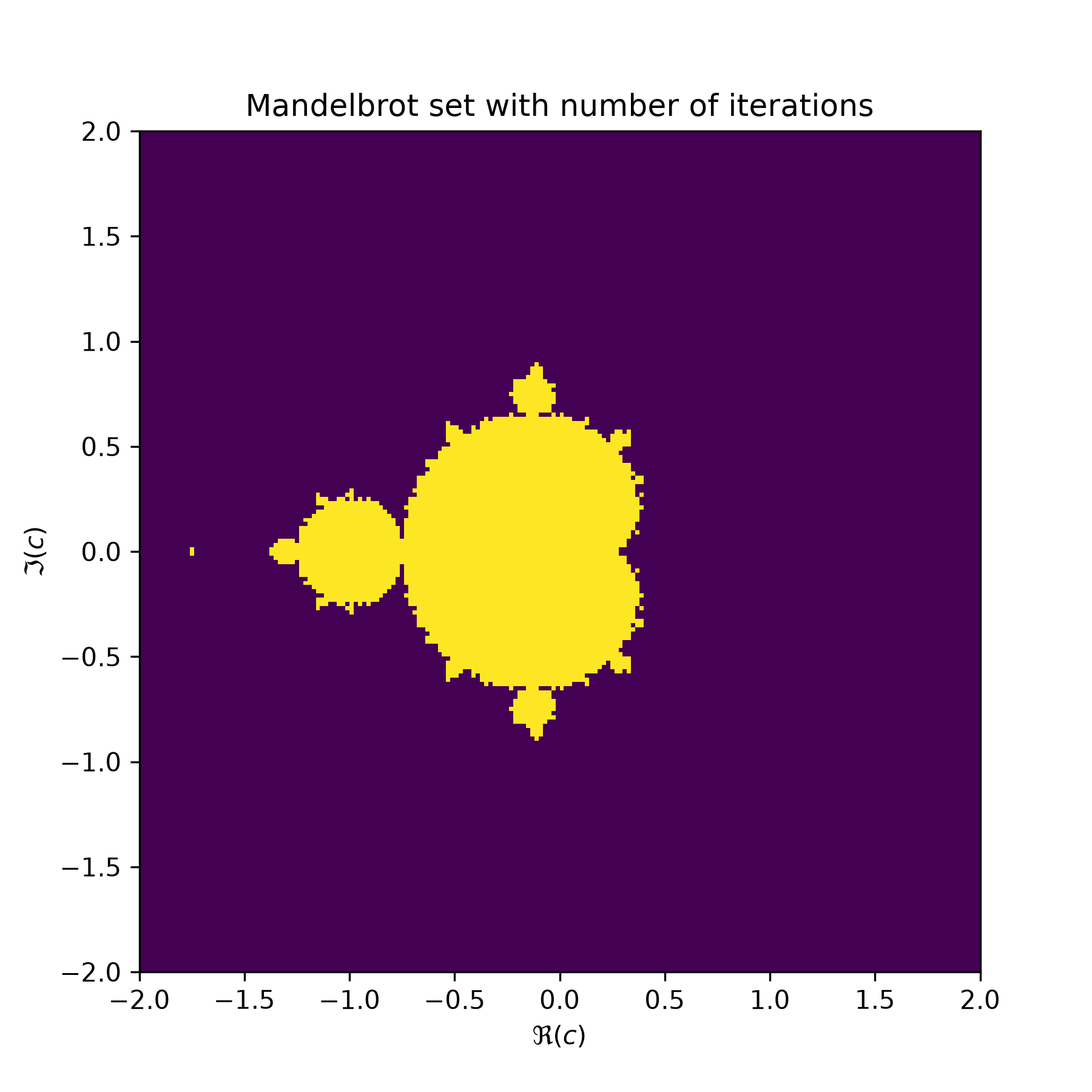
d. Using the previous function with \(N=100\), plot with imshow an approximation of the set of points belonging to the Mandelbrot set.

e. Adapting the previous functions, plot the logarithm of the number of iterations required before \(|z_n|\leq 2\) is no longer satisfied instead of a Boolean, as represented in Figure 4.5.

f. !! The previous method has the disadvantage of computing each value of \(c\) sequentially, which makes the evaluation rather slow. Propose a new implementation allowing to compute in parallel all the values using NumPy indexing.

Exercise 4.4 - Advanced graphics !

The purpose of this exercise is to discover a range of possibilities offered by Matplotlib.

a. Draw the stream lines of the vector field of the Van der Pol oscillator:

\[\begin{pmatrix}y\\ -x+\mu(1-x^{2})y \end{pmatrix}\]

for different values of \(\mu\in\mathbb{R}\).

b. Plot the parametric curve:

\[\begin{pmatrix}\left(1+t^{2}\right)\sin(2\pi t)\\ \left(1+t^{2}\right)\cos(2\pi t)\\ t \end{pmatrix}\]

for \(t\in[-2,2]\).

c. Plot the function of two variables:

\[ f(x,y)=\sin\left(\sqrt{x^{2}+y^{2}}\right) \]

in three dimensions for \(x\in[-5.5]\) and \(y\in[-5.5]\).

d. !! Represent the given Möbius strip as a parametric surface:

\[\begin{pmatrix}\left(3+v\cos(u/2)\right)\cos u\\ \left(3+v\cos(u/2)\right)\sin u\\ v\sin(u/2) \end{pmatrix}\]

for \(u\in[0,2\pi]\) and \(v\in[-1,1]\).

e. !! Look at the examples available here and choose two to understand and modify.