8  Symbolic calculation

Exercise 8.1 - Introduction to SymPy

Before you can use symbolic variables, you have to declare them as symbols:

x = sp.Symbol("x") # define the symbol x
y = sp.Symbol("y", real=True) # define a real varaible y
e = sp.Symbol(r"\varepsilon", real=True, positive=True) # define a positive variable

Then, it is possible to perform operations between symbols:

x + 2*y + e/4 + x**2 + 3*x + 2*y

Most of the mathematical functions are implemented symbolically in SymPy and it is also possible to simplify them:

expr = sp.cos(x)**2 + sp.sin(x)**2 + (y**3 + y**2 - y - 1)/(y**2 + 2*y + 1) + sp.exp(-e)
sp.simplify(expr)

Finally, it is possible to make substitutions:

expr.subs(x,y) # substitute x by y
expr.subs({y:x, e:y}) # substitute y by x and e by y

then, for example, simplify the expression and plot its graph as a function of x as in Figure 8.1:

f = sp.simplify(expr.subs({y:x, e:y}))
sp.plot(f,(x,-2,6), title=f"Plot of ${sp.latex(f)}$")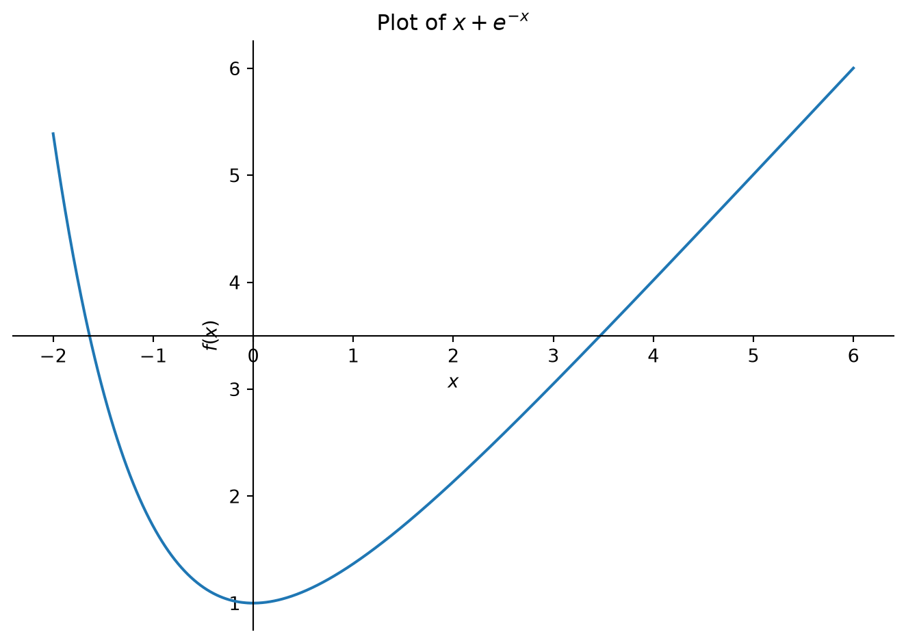

a. Read the documentation for the solve function and use it to calculate the roots of a general polynomial of degree two, then of degree three.

b. Read the documentation for the functions evalf and N to evaluate numerically the expression \(\frac{\pi^2}{4}\).

c. Read the documentation for the Rational function and numerically evaluate the rational number \(\frac{43609}{999}\) to 50 decimal places.

d. Determine the real and imaginary part of the expression:

\[ \bigg(\frac{1+i\sqrt{3}}{1+i}\bigg)^{20} \,. \]

e. Read the documentation for the function diff and calculate the derivative of \(x e^{x^{x^x}}\) with respect to \(x\).

f. Read the documentation of the function integrate and calculate the following integrals:

\[ \begin{align*} I_{1} & =\int x^{5}\sin(x)\,\mathrm{d} x \,, & I_{2} & =\int_{0}^{\infty}\sin(x^{2})\,\mathrm{d} x \,. \end{align*} \]

g. Calculate with SymPy the following limits:

\[ \begin{align*} L_{1} & =\lim_{x\to0}\frac{\sin(x)}{x}\,, & L_{2} & =\lim_{x\to0}\sin\bigg(\frac{1}{x}\bigg)\,, & L_{3} & =\lim_{x\to\infty}\frac{5x^{2}+3x+2y}{y(x-4)(x-y)}\,. \end{align*} \]

h. Compute the series expansion of \(\tan(x)\) at \(x=0\) to order 10 and the asymptotic expansion of \(\left(1 + \frac{1}{n}\right)^n\) for \(n\to\infty\) to order 5.

i. Determine the eigenvalues of the matrix:

\[\begin{pmatrix}1 & a & 0\\ a & 2 & a\\ 0 & a & 3 \end{pmatrix} .\]

Exercise 8.2 - Applications

The goal is to use SymPy to solve symbolically different mathematical problems by calculating the least possible things by hand.

a. Determine the number of zeros in the integer \(123!\).

b. Determine the ratio between the height and radius of a cylinder so as to minimize its area at a fixed volume.

c. For \(x,y\in\mathbb{R}\) such that \(xy < 1\), show that

\[ \arctan(x) + \arctan(y) = \arctan\left(\frac{x+y}{1-xy}\right) \,. \]

d. Prove the following formula due to Gauss:

\[ \frac{\pi}{4} = 12\arctan\left(\frac{1}{38}\right)+20\arctan\left(\frac{1}{57}\right)+7\arctan\left(\frac{1}{239}\right)+24\arctan\left(\frac{1}{268}\right) \,. \]

It is imperative to use SymPy, the original demonstration of Gauss being 25 pages long, see pages 477 to 502 of the second volume of his complete works available here.

e. Determine the volume of the region:

\[ \big\{(x,y,z)\in\mathbb{R}^3: x^2+y^2 < z < 2x^2+4xy+6y^2, |y| < 5, |x| < 4\big\} \,. \]

f. Determine the expression of the real Fourier coefficients of the \(2\pi\)-periodic function \(f\) defined by \(f(x)=|\sin(x)|\).

Exercise 8.3 - Conjecture due to Euler

Euler conjectured in 1769 that at least \(k\) powers of strictly positive integers are necessary for the sum to be itself a \(k\) power. In other words, if \(n \geq 2\), \(k \geq 1\), \(a_1,a_2,\dots,a_n \geq 1\) and \(b \geq 1\) are integers such that:

\[ \sum_{i=1}^{n}(a_i)^k = b^k \]

then necessarily \(n \geq k\). This conjecture was disproved in 1966 by Lander & Parkin (doi:10.1090/S0002-9904-1966-11654-3) in what appears to be the shortest mathematical paper ever written with a counterexample for \(k=5\):

\[ 27^5 + 84^5 + 110^5 + 133^5 = 144^5 \,. \]

The goal is to show that this counterexample is the simplest possible, in the sense that it is the only counterexample with \(k \leq 5\) and \(b \leq 144\).

a. Show that Euler’s conjecture is true for \(k=1\) and \(k=2\).

b. Check with Python the above counterexample.

c. Write a function powers(bmax,k) that returns the set (type set) of all integers from 1 to bmax raised to the power k.

d. Check that there is no counterexample with \(k=3\) and \(b \leq 144\).

e. Write a function combinations(lst,n) that for a list of integers lst and an integer n returns the list of all combinations of n integers in lst in ascending order. For example, combinations([1,2,3,4],2) should return [(1,1), (1,2), (1,3), (1,4), (2,2), (2,3), (2,4), (3,3), (3,4), (4,4)].

f. Write a function test(bmax,n,k) that for three given integers bmax, n, and k, iterates over all combinations of n integers returned by combinations and checks whether the sum of these n integers raised to the power k is an integer present in the list powers(bmax,k). Use this function to check that there is no counterexample to Euler’s conjecture for \(k=4\) and \(b \leq 144\). Depending on the power of your computer, it is possible to choose also \(k=5\) and thus to check that the counterexample of the introduction is indeed the simplest one.

For \(k=5\), the previous method of iterating over all combinations is rather slow. A faster method is to observe that the set of sums of type:

\[ (a_1)^5 + (a_2)^5 + (a_3)^5 + (a_4)^5 \,, \]

can be written as \(S_1 + S_2\) where \(S_1\) and \(S_2\) are sums of two integers to the power 5.

g. Write a function sum2(bmax,k) which returns a dictionary having for keys the sums \((a_1)^k+(a_2)^k\) with the associated value \((a_1,a_2)\) for \(0 \leq a_1 \leq a_2 \leq\) bmax. We will take care to remove the trivial element zero from the dictionary. When building the dictionary, make sure that it is uniquely defined in the sense that there is no other possible value for an existing key. Test sum2(300,5) and sum2(300,3).

h. Use the dictionary constructed earlier to determine the set of counterexamples for \(k=5\) and \(b \leq 300\) by iterating over all elements of powers(bmax,5) and sum2(bmax,5).

Exercise 8.4 - Pathological function

The goal is to construct a function that visually looks regular, but in fact is not. Let the function \(f:\mathbb{R}\to\mathbb{R}\) be defined by:

\[ f(x) = \sum_{k=1}^{\infty} \frac{\sin(k^2 x)}{k^5} \,. \]

Since the series converges absolutely, the function \(f\) is well defined.

a. With the help of SymPy calculate the function \(g:\mathbb{R}\) defined by keeping the first hundred terms of the series:

\[ g(x) = \sum_{k=1}^{100} \frac{\sin(k^2 x)}{k^5} \,, \]

and plot the function \(g\).

b. Estimate by hand the error between the functions \(f\) and \(g\) in absolute value.

c. Calculate the first derivative and the second derivative of \(g\) and plot these two derivatives. What can you conclude?

d. Explain mathematically what is going on.

Exercise 8.5 - Green’s function of the Laplacian !

The goal of this exercise is to compute fully automatically the Green’s function of the Laplacian in \(\mathbb{R}^3\), i.e., the solution satisfying:

\[ \Delta G(\boldsymbol{x}) = \delta(\boldsymbol{x}) \,, \]

in \(\mathbb{R}^3\), where \(\delta(\boldsymbol{x})\) is the Dirac distribution.

For this, we introduce the spherical coordinates \(\boldsymbol{x}^\prime = (r,\theta,\varphi)\) with \(r>0\), \(0 \leq \theta \leq \pi\) and \(0 \leq \varphi < 2\pi\) characterized by:

\[ \begin{align*} x_1 & =r\cos\varphi\sin\theta\\ x_2 & =r\sin\varphi\sin\theta\\ x_3 & =r\cos\theta \,. \end{align*} \]

a. Define a function to_spherical(expr) to convert an expression given in Cartesian coordinates to spherical coordinates.

b. Define a function to_cartesian(expr) allowing to convert into cartesian coordinates an expression given in spherical coordinates. For simplicity, we can only deal with the case of an expression expr invoking the variables \(r\) and \(\theta\) but not \(\varphi\).

c. Calculate the scale factors of the spherical coordinates:

\[ h_i = \left\Vert \frac{\partial\boldsymbol{x}}{\partial x^\prime_i} \right\Vert. \]

d. Define a function gradient(f) allowing to calculate the gradient of a function \(f:\mathbb{R}^3\to\mathbb{R}\) in spherical coordinates:

\[ \boldsymbol{\nabla}f = \left( \frac{1}{h_i}\frac{\partial f}{\partial x^\prime_i} \right)_{i=1}^3\,. \]

e. Do the same to define the Laplacian in spherical coordinates:

\[ \Delta f = \sum_{i=1}^3 \frac{1}{J} \frac{\partial}{\partial x^\prime_i} \left( \frac{J}{h_i^2} \frac{\partial f}{\partial x^\prime_i} \right) \quad \text{where} \quad J = \prod_{i=1}^3 h_i \,. \]

f. Find the radial solutions (i.e., depending only on the variable \(r\)) of the equation \(\Delta G = 0\) in \(\mathbb{R}^3\setminus\{\boldsymbol{0}\}\).

g. Determine the equations that the integration constants must satisfy for the above solution to satisfy in Cartesian coordinates:

\[ \lim_{|\boldsymbol{x}|\to\infty} G(\boldsymbol{x}) = 0 \quad \text{and} \quad \Delta G(\boldsymbol{x}) = \delta(\boldsymbol{x}) \,. \]

h. Solve the equations on the integration constants and substitute in the radial solution of \(\Delta G = 0\) to obtain the expression of the Green’s function of the laplacian in spherical coordinates. Finally, determine the Green’s function \(G\) of the Laplacian in \(\mathbb{R}^3\) in Cartesian coordinates.

i. !! Let \(g:\mathbb{R}^3 \to \mathbb{R}\) be a smooth function with compact support invariant by rotations along the vertical axis. Determine the asymptotic behavior at large distances of the solution of the equation:

\[ \Delta f(\boldsymbol{x}) = g(\boldsymbol{x}) \, \]

up to order two, i.e., the terms decreasing as \(|\boldsymbol{x}|^{-1}\) and as \(|\boldsymbol{x}|^{-2}\).