10  Probability and statistics

Exercise 10.1 - Harmonic series of random sign

The goal of this exercise is to simulate the convergence of a harmonic series whose sign is drawn randomly. More precisely, if \((X_i)_{i\in\mathbb{N}}\) is a sequence of independent random variables worth \(-1\) or \(1\) with probability \(\frac{1}{2}\), then we define the partial sum:

\[ W_0 = 0 \,, \qquad\qquad W_n = \sum_{i=1}^n \frac{X_i}{i} \,, \]

and the question is to determine if the sequence \((W_n)_{n\in\mathbb{N}}\) converges and if so toward what.

a. Write a function sign() that simulates the random variable \(X_i\).

b. Write a function simulate(n) that returns a realization of \((W_0,W_1,\dots,W_n)\).

c. Plot the function \(n \mapsto W_n\) for different realizations, for example, for \(0\leq n\leq 1 000\) and make a conjecture about the convergence of the sequence \((W_n)_{n\in\mathbb{N}}\).

d. ! Determine the histogram of \(W_{1 000}\) for \(10^4\) or \(10^5\) realizations to get an idea of the law of the limiting random variable.

Exercise 10.2 - Gambler’s ruin

The goal is to simulate the evolution of the amount of money of a gambler playing heads or tails. At each toss, the player wins one euro if it is heads and loses one if it is tails. The probability of getting tails is noted \(p\), that of getting heads \(q\). In particular, \(p=q=\frac{1}{2}\) if the coin is balanced.

Mathematically, the sum \(S_i\) owned by the player at time \(i\) is given by a random walk:

\[ S_{i}=\begin{cases} 0\,, & \text{if}\:S_{i-1}=0\,,\\ S_{i-1}+X_{i}\,, & \text{if}\:S_{i-1}\geq1\,, \end{cases} \]

where \((X_i)_ {i}\) are independent random variables of law \(\mathbb{P}(X_i=1) = p\) and \(\mathbb{P}(X_i=-1) = q\).

a. Write a function simulate(p,k,N) that generates a realization of length \(N\) of the process from \(S_0=k\), i.e., returns \((S_0,S_1,S_2,\dots,S_N)\). Represent graphically several realizations.

b. Simulate a player who, starting with a sum \(k\), plays until he loses everything or has the amount \(n \geq k\).

c. If \(T\) is the time at which the game stops, i.e., when \(S_T = 0\) or \(S_T = n\), recover by simulation the theoretical results on the average time:

\[ \mathbb{E}(T)=\begin{cases} k(n-k)\,, & \text{if}\:p=q\,,\\ \dfrac{n}{p-q}\dfrac{1-\rho^{k}}{1-\rho^{n}}-\dfrac{k}{p-q}\,, & \text{if}\:p\neq q\,, \end{cases} \]

and the place of exit:

\[ \mathbb{P}(S_{T}=0)=\begin{cases} \dfrac{n-k}{n}\,, & \text{if}\:p=q\,,\\[4pt] \dfrac{\rho^{k}-\rho^{n}}{1-\rho^{n}}\,, & \text{if}\:p\neq q\,, \end{cases} \]

where \(\rho = q/p\). For this, we can plot these quantities as a function of \(p\) or just consider the case \(p=q=\frac{1}{2}\).

Exercise 10.3 - Pólya urn

An urn initially contains (at \(t=0\)) \(r_0\) red balls and \(b_0\) white balls. At each time, we pick a ball uniformly at random from the urn. This ball is then returned to the urn and a ball of the same color is added. Such a system is called a Pólya urn. The purpose of this exercise is to study the behavior of the fraction of red balls in the urn, i.e., the number of red balls out of the total number. We will call \(r_n\) and \(b_n\), respectively, the number of red and white balls in the urn at time \(n\).

a. Write a function density taking as argument a tuple representing the number of red and white balls in an urn, and which returns the density of red balls.

We want to recursively construct the distribution of the number of red balls at time \(n\), i.e., the list of probabilities that the number of red balls is equal to a given integer \(k\) (which will be the index of the list). This is done by writing two functions: next_dist_red, which takes as argument the distribution at time \(n\) and returns the one at time \(n+1\), which is thus the function that does all the work, and dist_red, which is the wrapper function, taking as argument \(r_0\), \(b_0\), and time \(n\) and returning the distribution at time \(n\) by a recursive call. We will use the following useful facts (make a small drawing):

• The distribution passed as an argument to next_dist_red is a list r, and r[k] represents the probability of having k red balls in the urn at time \(n\). The indices for r vary from 0 to the total number s of balls at time \(n\).
• At time \(n+1\), to have \(k\) red balls, we need:
  • either having had \(k\) red balls at the previous time and not having drawn a red ball;
  • or having had \(k-1\) red balls at the previous time and having drawn a red ball.
• If \(n=0\), the result of dist_red is completely deterministic and the coefficients of the list are only 0 and 1, depending on \(r_0\) and \(b_0\).

b. Write the functions next_dist_red and dist_red using the directions provided. Look at the result of dist_red(0,1,n) and dist_red(1,1,n) for different values of n \((1,2,5,10,20,\dots)\) and comment.

Rather than theoretically computing for each \(n\) the sequence of theoretical probabilities, we will do statistics on a large number of Pólya urn realizations, after a large number of steps. For this, we need a function to evolve a Pólya urn.

c. Define a function polya_step(r,b) which, given the composition of an urn passed as two parameters r and b, returns the (random) evolution after one step of the composition of the urn as a tuple. Also define a function polya(r0,b0,N) taking as arguments \(r_0\), \(b_0\) and \(N\) as parameters and returning the (random) composition of a Pólya urn after \(N\) steps, also as a tuple.

d. Write a function data_rdens_polya(r0,b0,N,nbexp) that returns a list of length nbexp containing the densities of nbexp realizations of Pólya urns at time N initialized with r0 red balls and b0 white balls.

e. Store the result of data_rdens_polya(2,3,1000,10_000) in a variable and draw a histogram to see the distribution of densities. Be careful, we want the heights of the bars to be normalized so that their surface represents the proportion of points, and not so that they give the number of points per bin.

Exercise 10.4 - Central limit theorem

The central limit theorem (also known as the central limit theorem, the central limit theorem or the central limit theorem) establishes the convergence of the sum of a sequence of random variables toward the normal distribution. Intuitively, this result states that a sum of identical and independent random variables tends (under certain conditions) toward a Gaussian random variable. Here’s how it works:

Theorem: Let \((X_n)\) be a sequence of independent real random variables of the same distribution with expectation \(\mu\) and standard deviation \(\sigma \ne 0\). Let \((\bar{X}_n)\) be the sequence defined by:

\[ \bar{X}_n = \frac{1}{n} \sum_{k=1}^n X_k \,. \]

For \(n\) large enough, the distribution of \(\bar{X}_n\) can be approximated by the normal distribution \(\mathcal{N}(\mu, \frac{\sigma^2}{n})\).

The aim of this exercise is to check whether this theorem is valid for different laws of probability:

• Poisson distribution: discrete distribution on \(\mathbb{N}\), of parameter \(\lambda\), defined by:

\[ \mathbb{P}(X = k) = \exp(-\lambda) \frac{\lambda^k}{k!}\,, \quad \forall k \in \mathbb{N} \,. \]

• Normal distribution: continuous distribution on \(\mathbb{R}\), of parameters \(m\) and \(\sigma\), defined by density:

\[ \frac{1}{\sqrt{2\pi\sigma^2}} \exp\left( - \frac{(x-m)^2}{2\sigma^2} \right)\,, \quad \forall x \in \mathbb{R} \,. \]

• Cauchy distribution: continuous distribution on \(\mathbb{R}\), of parameters \(a\) and \(\gamma\), defined by density:

\[ \frac{1}{\pi\gamma\left(1 + \left(\frac{x-a}{\gamma}\right)^2\right)}\,, \quad \forall x \in \mathbb{R} \,. \]

a. Define a function normal_density(x, mu var) taking as an argument :

• x (array): an array of floating-point numbers;
• mu (floating number): average \(\mu\);
• var (strictly positive floating number): variance \(\sigma^2\);

and which returns the density of the normal distribution evaluated for each number \(x\) in x:

\[ \mathcal{N}(\mu, \sigma^2) = \frac{1}{\sqrt{2\pi\sigma^2}} \exp\left( - \frac{(x-\mu)^2}{2\sigma^2} \right) \,. \]

b. Look at the documentation for the numpy.random.poisson function and generate 10 random values according to a Poisson distribution with parameter \(\lambda = 2\).

c. Write a function samples_poisson(lam, N, M) which takes as arguments:

• lam (strictly positive real): parameter \(\lambda\) for the Poisson distribution;
• N (strictly positive integer): number of experiments;
• M (strictly positive integer): number of random variables generated for each experiment;

and which generates N experiments with M random variables generated per experiment, and returns:

• the average value (floating number) over the N * M random variables generated;
• the standard deviation (floating number) on the N * M random variables generated;
• a numpy vector of size N where each element is the mean of the random variables in an experiment.

For the values lam=2 and N=10_000, run samples_poisson(lam, N, M) for \(M \in \{10, 100, 1 000\}\) and save the results in variables.

d. For each value of M, display the distribution of the numpy vector containing the means of each experiment, as well as the distribution of the expected normal distribution if the central limit theorem is verified. You can use Matplotlib hist function to display the histogram of a table, with the bins=50 parameter to set the number of columns and density=True to display a probability distribution. Use the empirical means and standard deviations returned by the samples_poisson function for normal distribution parameters. Choose relevant values for the x-axis boundary values. Make a hypothesis on the validity of the central limit theorem for the Poisson distribution.

e. Repeat questions c) and d) for the normal distribution. Using the function numpy.random.normal, generate averages for loc=2, scale=1, N=10_000, and \(M \in \{10, 100, 1 000\}\). Plot the histograms and make a hypothesis about the validity of the central limit theorem for the normal distribution.

f. Repeat questions c) and d) for the Cauchy distribution with \(a=0\) and \(\gamma=1\). To do this, use the function numpy.random.standard_cauchy. Use bins=np.arange(-10, 10.1, 0.1) and make an assumption about the validity of the central limit theorem for the Cauchy distribution.

Exercise 10.5 - Random generation of unit vectors

The aim of this exercise is to find an efficient method for randomly generating unit vectors in \(\mathbb{R}^n\) according to a uniform distribution. We will start with the case \(n = 2\), where a real vector can be represented by a complex number.

a. Consider the following strategy for randomly generating a unit vector in \(\mathbb{R}^2\):

1. Generate \(x\) randomly according to the uniform distribution on \([-1, 1]\);

1. Generate \(y\) randomly according to the uniform distribution on \([-1, 1]\);

1. Return the unit complex \(z = \frac{x}{\sqrt{x^2 + y^2}} + \frac{y}{\sqrt{x^2 + y^2}}i\).

Write a function generate_complex which takes as argument a positive integer \(N\) and returns a NumPy array of size \(N\), where each element is a complex generated by the above strategy.

b. For \(n=2\), one way to check whether the distribution of vectors is uniform is to look at the distribution of angles/arguments of the complex numbers (i.e., \(\arg{z}\)): this should be uniform. Use the generate_complex function with \(N = 10^6\) and display the distribution of angles/arguments. Does the strategy described in the previous question generate unit vectors uniformly?

c. The following modification to the previous strategy is proposed:

1. Generate \(x\) randomly according to the uniform distribution on \([-1, 1]\);

1. Generate \(y\) randomly according to the uniform distribution on \([-1, 1]\);

1. If \(x^2 + y^2 \leq 1\), return the unit complex \(z = \frac{x}{\sqrt{x^2 + y^2}} + \frac{y}{\sqrt{x^2 + y^2}}i\) (otherwise return nothing at all).

Write a function generate_complex_monte_carlo which takes as argument a positive integer \(N\) corresponding to the number of candidate vectors and returns a NumPy array of size \(n \leq N\), where each element is a complex generated by the above strategy. Warning: \(n\) is random and therefore cannot be determined in advance.

Repeat the previous question and display the angle/argument distribution of the complexes generated by this strategy. Does this strategy generate unit vectors uniformly?

d. We now ask how many candidate complexes must be generated on average to accept \(n\) of them, which is equivalent to determining how many complexes are accepted on average from the \(N\) candidates. The law of large numbers means that the ratio converges to the probability that a candidate vector will be accepted. This probability is equal to the ratio of the inclusion area \(\pi\) (the unit circle) to the total area \(4\) (the square \([-1, 1]^2\)), i.e., \(\frac{\pi}{4}\). Compare the ratio \(\frac{n}{N}\) to \(\frac{\pi}{4}\).

e. We now consider the general case \(n \geq 2\). The strategy considered is the same as in question c):

1. Generate a vector \(\boldsymbol{x}=(x_1, \ldots, x_n)\), where each \(x_k\) is randomly and independently generated according to the uniform distribution on \([-1, 1]\);

1. If \(\Vert \boldsymbol{x} \Vert_2 \leq 1\), return the unit vector \(\frac{\boldsymbol{x}}{\Vert \boldsymbol{x} \Vert_2}\).

The volume of the unit ball in \(\mathbb{R}^n\) is given by:

\[ V_n = \frac{\pi^{n/2}}{\Gamma(\frac{n}{2} + 1)} \]

and the volume of the cube \([-1, 1]^n\) is \(2^n\). Plot the probability of a vector being accepted in step 2 of this strategy for \(n \in \{2, \ldots, 20\}\). Do you think this strategy is effective for large \(n\) values?

f. The following strategy can be shown to generate random vectors on \(\mathbb{R}^n\):

1. Generate a vector \(\boldsymbol{x}=(x_1, \ldots, x_n)\), where each \(x_k\) is generated randomly and independently according to the reduced centered normal distribution: \(x_k \sim \mathcal{N}(0, 1)\);
2. Return the unit vector \(\frac{\boldsymbol{x}}{\Vert \boldsymbol{x} \Vert_2}\).

Verify for \(n=2\) that this strategy does indeed randomly generate unit vectors according to a uniform distribution by displaying the angle distribution (representing the vectors as complex numbers) for \(N = 10^6\) vectors.

Exercise 10.6 - Percolation !!

The goal is to study a percolation model in a porous medium. The medium is modeled by a random matrix of Booleans that determines which sites can be invaded by water and which are impermeable. A matrix percolates if there is a water path from the top row to the bottom row. In the examples in Figure 10.1, the entries of a matrix that can be percolated are colored and the entries that are actually filled with water are in blue. The first matrix does not percolate while the second does.

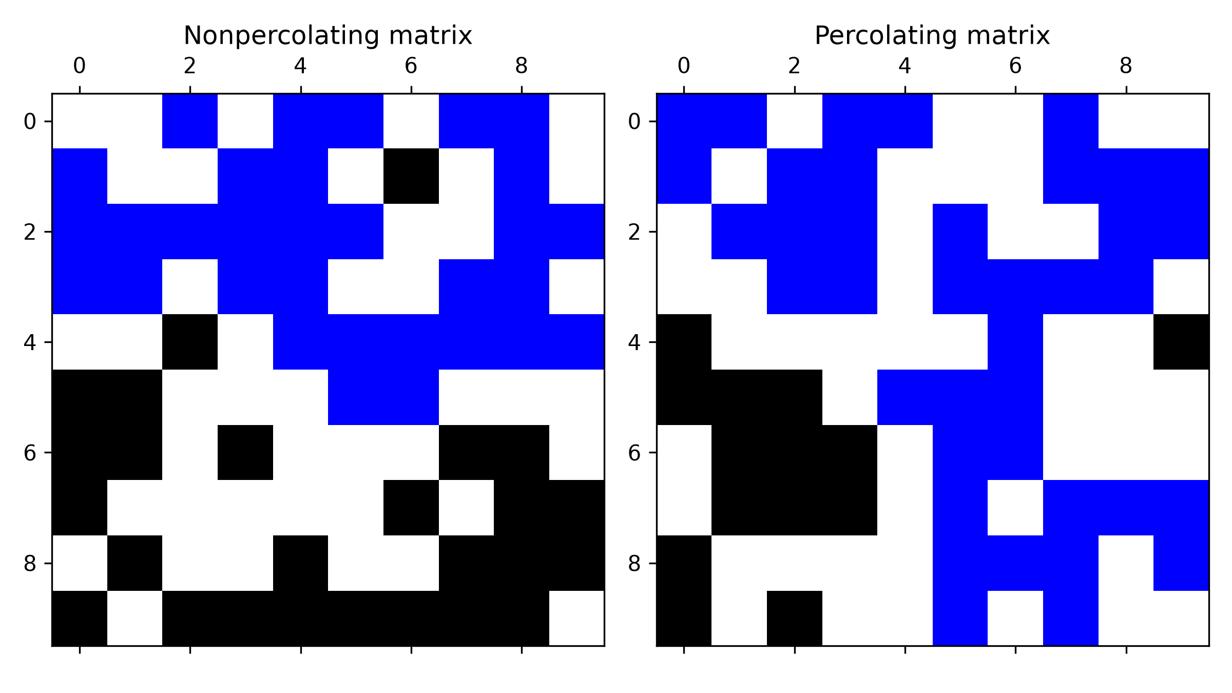
a. Write a function generate(n,p) that generates a matrix of Booleans of size \(n \times n\) such that each entry has probability \(p\) of being right and \(1-p\) of being wrong.

b. Define a function fill(isopen) that for a given Boolean matrix returns another Boolean matrix with the entries invaded by water.

c. Using Matplotlib, represent the filling of different randomly generated matrices.

d. Define a function percolate(isopen) to determine whether a Boolean matrix is percolating or not.

e. !! Calculate the time needed to determine if a matrix of size \(50 \times 50\) with \(p=0.9\) is percolating or not. Read the documentation of the Numba module to reduce the calculation time by compiling one of the functions: https://numba.pydata.org/.

f. By doing statistics, determine the probability that a Boolean random matrix of size \(n \times n\) with probability \(p\) will percolate. Study this probability as a function of \(p\) and \(n\).

g. !!! The statistics performed in the previous point are a typical example of calculations that can be easily executed in parallel, because each case is independent of the others. Parallelize the previous algorithm in such a way as to use all the cores of your processor, for example, with the help of the module mpi4py.